Leeham News and Analysis
There's more to real news than a news release.

Bjorn’s Corner: Aircraft drag reduction, Part 12

By Bjorn Fehrm
January 12, 2018, ©. Leeham Co: In the last Corner, we described how the theory for the boundary layer was proposed by Ludwig Prandtl, and how this led to an understanding of the source of Friction drag for an aircraft.
We will now continue with describing how the role of Friction drag was researched and how aircraft designers learned how to reduce it.

Figure 1. Sopwith Camel fighter of the WW 1. Source: Google images.
Friction drag
In his paper of 1904, Prandtl (Professor at the Technical University of Hanover at the time) not only presented the theory of how the friction of air against a surface would create a boundary layer and with it Friction drag, he also suggested how the Friction drag could be calculated from the complicated Navier-Stokes equations.
He presented how the equations could be simplified for the shallow area of two-dimensional flow within the boundary layer and therefore solved.
Four years later, one of his students, Heinrich Blasius, presented a paper which reduced the complex equations further, now to a normal differential equation. The equations, which are used still today, are called the Blasius equations.
Until the 1930s, the aircraft were flying at low speeds as the Form drag from the wires and braces on the aircraft (Figure 1) was huge and the aircraft had high induced drag. The short wings were used during the war to make the aircraft agile in roll. While giving more drag, rolling fast to avoid an enemy attack was more important than fuel efficiency and speed.
Gradually, the Form drag of the aircraft decreased and the designers understood; to go faster the amount of surface area that scrubbed the air, causing Friction drag, should be reduced. Measurements were now done in wind tunnels on how different types of form and area affect the Friction drag. One found that dependent on airspeed and test object size, there were essentially two drag curves for friction drag, Figure 2.
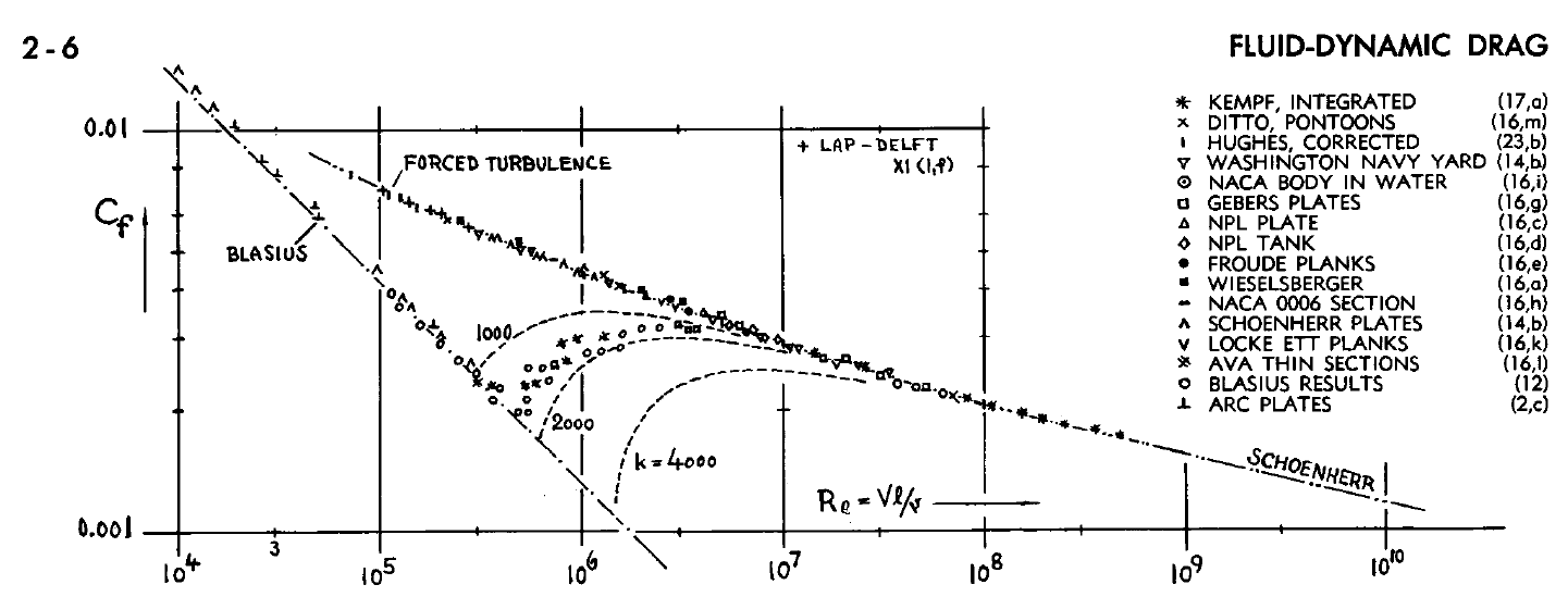
Figure 2. Friction drag per unit area (Cf) as a function of airspeed (V), object length (l) and viscosity (v). Together these form the Reynolds number Re. Source: Hoerner, Fluid dynamic drag.
At low airspeed the drag was low (left curve in Figure 2). If speed was increased, the drag jumped to the higher curve. Gradually, one understood the first curve was for an orderly flowing boundary layer with laminar flow. The higher drag curve was for a boundary layer which had switched to turbulent flow.
The transition point both in speed and position on the test object (flow starts as laminar and then changes to turbulent after less than 20% distance of the test object) was not consistent. Dependent on surface finish and the test items size compared to the airspeed, it happened at lower or higher flow speeds. And dependent on surface smoothness it happened after approximately 10% of the object’s length or later One understood it depended on how the fluid’s viscosity (stickiness) compared to the airspeed and to the size of the object the air should flow around. One had discovered the Reynolds number effects.
The Reynolds number says: to have a comparable result of scale model tests to full-size tests, the Reynolds number between the test shall be the same.
This means if the model of an aircraft is half the size of the real aircraft, you need to double the airspeed in the tunnel. Or double the density or half the viscosity. This is what was done by NACA in the 1920s. Increasing tunnel speed to the area of Re 10^6 to avoid the change area from laminar to turbulent flow and to get the Re close to full-size aircraft Re (between 10^6 and 10^7) required enormous fans. Instead, the wind tunnel was placed in a pressure chamber where the density could be increased by increasing the air pressure. The best model results at the time came from this NACA wind tunnel, as it could reach the highest Re number, coming close to real-world Re.
It was recognised it was difficult to keep the flow laminar over any length of an aircraft surface. The tiniest unevenness of the surface would trigger turbulent flow at the Re numbers the aircraft flew at. Laminar flow friction drag was therefore ignored until NACA developed a series of airfoil types before WW 2, which kept the flow laminar over a longer distance from the leading edge of the wing, thereby reducing Friction drag. The P51 Mustang was designed with such a wing profile.
With classical aluminum manufacturing methods, the forward wing area could not be kept smooth enough, so there wasn’t much laminar flow over the Mustang wing. Yet, it had low high-speed drag? Yes, because the wing profile for laminar flow is close to a transonic wing profile. The Mustang designers had reduced high-speed transonic drag without knowing it. Transonic drag wasn’t understood until after WW 2. We will cover this in a subsequent Corner.
Wing lift theory and induced drag
Between 1908 and 1920, Prandtl and the Göttingen team could develop a practical theory and formulas for wing lift on finite span wings. It was based on the infinite span formula developed by Professor Nikolai Zhukovsky of the Imperial Technical School of Moscow (called the Kutta-Joukowski theory). This theory also outlined how induced drag affected the wing, which is the subject for our next Corner.
By now the aircraft designers knew, to make an efficient and fast aircraft one should:
- Minimize the surface area of the aircraft to avoid excessive Friction drag (called the wetted area as it’s the area which is wetted by the airstream).
- Avoid wires and braces for structural strength and blunt aft bodies, as these create separation and therefore Form drag.
- Give the wing a high span to avoid induced drag. As the wetted area of the wing shall be kept low to reduce Friction drag, the requirement is; high span and low area, which translates to high aspect ratio (Aspect ratio = span^2/wing area)
Thanks Bjorn. You once had post relating to fuselage width and length relating to “wetted area” per pax. With the NMA, A322, etc discussions going on I think very interesting/important subject. Can recall something that change over from 3-3 to 2-3-2 is around 230 pax and to 2-4-2 around 270/280, etc?
Will be nice if you could “publish” it again, can’t find it (my admin about 1/10).
Another trick is to lower the gas temperature in the wind tunnel.
Fundamentally, if the temperature of the flow is decreased, the viscosity of the gas and the velocity of sound decrease and the density increases. The overall effect of cooling is that the Reynolds number increases rapidly. Thus a pressurized tunnel at very low “cryogenic” temperatures can provide real-flight Reynolds numbers by virtue of both increased pressure and decreased temperature.
In ETW the models are not tested in an air stream, as is the case in conventional wind tunnels. Instead, a pure nitrogen flow with a temperature down to 110 Kelvin (= -163°C = -261°F).
Thanks, although I studied Physics and Chemistry at University as pax the aerodynamic aspects never crossed my mind, you just think that its bloody cold out there. Air temperatures generally -40 t0 -50C at around 35K feet.
When working with liquid Nitrogen in the wind tunnel what is the impact of the air’s moisture content in creating “induced turbulence”?
The N2 is not liquid after it fills the tunnel sections. Still it needs cooling due to heating from operation and heat transfer. Do not know what remaining moisture there is in the wind tunnel after fill-up with N2. In real flight operations you can get icing problems at quite high altitudes as some modern Engines has had problems with ice build up at altitude and shredding Before modifications were incorporated.
Can recall reading about at least one close call at LHR of a BA 777 resulting from engine icing.
Heard Boeing is working on something to “see” clear sky turbulence, any idea how it works? Had some bad experiences and got respect for an A330’s wing (and wing box). Seems even in the modern day pilots rely on info from other aircraft in the area to find a suitable FL in these conditions.
Great explaining of difficult physics. Thanks Björn!
Until the 1930s, the aircraft were flying at low speeds as …
That was actually deviated from well before 1918.
Junkers “Blechesel” J1 shew that an unbraced high aspect ration wing provided greatly improved performance … for civil use. Base for worldwide success of the Junkers F13 and the Junkers airframes after that.
The interesting thing is that Junkers had the deep theoretical understanding ( from his research and research by his peers) to get there.
( Just read a Hugo Junkers Biography while traveling 🙂